Sort Function
The SORT function rearranges the contents of a range or array in ascending or descending order. It’s dynamic—if your source data changes, the sorted result updates automatically.
Picture

Syntax
=SORT(array, [sort_index], [sort_order], [by_col])
Argument
Array –The range or array to sort. (Required)
Sort_index – The column (or row) number within array to sort by. Defaults to 1. (Optional)
Sort_order – 1 = ascending (default), -1 = descending. (Optional)
By_col –FALSE (default) = sort by rows; TRUE = sort by columns. (Optional)
How To Use It
- Sort by the first column (ascending):
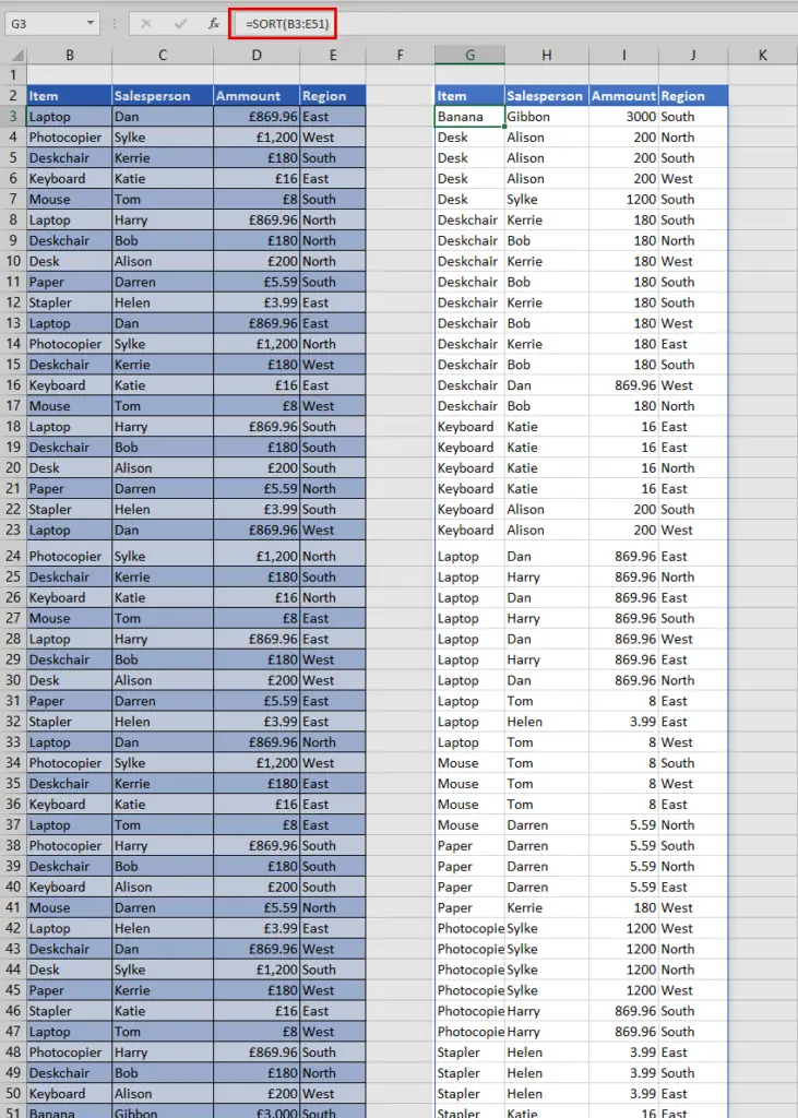
=SORT(B3:E51)
Sorts the entireB3:E51area by the first column in ascending order. - Sort by a specific column (ascending)
=SORT(B3:E51, 2, 1)Sorts the range by the 2nd column (e.g., Salesperson) in ascending order. Sort by a specific column (descending)
=SORT(B3:E51, 3, -1, FALSE)Sorts the range by the 3rd column (e.g., Amount) in descending order.FALSEconfirms sorting by rows.Combine with other functions:
=SORT(FILTER(B3:E51, B3:B51 = G3), 2, 1)First filters the table by a condition (e.g., item = “Laptop” inG3), then sorts the filtered result by column 2 in ascending order.
Why Use SORT?
Non‑destructive — leaves your original data intact while showing the sorted output elsewhere.
Dynamic updates — results spill and update automatically when data changes.
Easily integrated with other dynamic functions like
UNIQUE,FILTER, andSORTBY.
