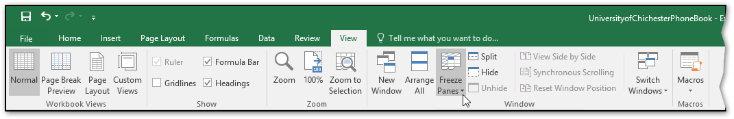
Freeze Panes

Freeze Panes

Freeze Panes can be used to lock specific columns or rows in place so that you may see them where-ever you are within the data. 

In the view tab of the ribbon you will find the "freeze panes" drop down menu:


This menu contains three options:


Freeze Top Row & Freeze First Column

The last two options in this menu will simply freeze in position of either the Top row or first column. These options are either selected or un-selected and will not work at the same time as the separate "Freeze panes" option.  Illustrative image


Freeze Panes (manually)

Keeps rows and columns visible while the rest of the worksheet scrolls, but will freeze anything above and to the left of the cell you have selected. In the image below you can see if I have selected cell "C2" and then when click the freeze panes button any rows above, or columns to the left, are frozen in position.

This means that everything above and to the left of Cell C2 will remain on screen at all times.  As shown in the image here.  Illustrative image

  1. Click the cell you wish to freeze everything that resides above or to the left of it. 
  2. Go to the view tab --> Freeze Panes --> Freeze panes. (This is also the same for unfreezing panes)  Illustrative image

Still need help?