Creating Pivot Tables in Excel #
Pivot tables are powerful tools for summarizing and analyzing data efficiently. They work best when your data is recorded in a “log format”
Each transaction listed individually without any pre-summed or aggregated totals. For example:
| Date | Sales Person | Product | Price |
| 13/12/2026 | Dan | Table | £110 |
| 14/12/2026 | Helen | Chair | £50 |
You don’t need to sum data before using a pivot table, Excel will do it for you in the Pivot table itself!
Step 1: Prepare Your Data #
- Make sure each column has a clear header.
- Avoid leaving entire rows or columns blank (a few empty cells are fine).
- Ensure your data is consistent and properly formatted.
- Check your dates formatting is working, convert dates to numbers, if the date does not change to a number. It may be stored as text.
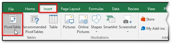
Step 2: Insert a Pivot Table #
There are two ways to start:
- Click any cell within your data, then go to Insert → PivotTable. Excel will automatically select the range.
- Alternatively, manually select your entire data range, then choose Insert → PivotTable. This lets you confirm the range and choose where to place the pivot table (usually a new worksheet).
Step 3: Choose Where to Place It #
In the PivotTable dialog box:
- Select New Worksheet (recommended) or Existing Worksheet.
- It’s recommended to use a new Worksheet, as it’s not always possible to know how much space the pivot table will use.
- Click OK.
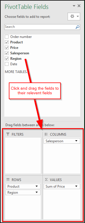
Step 4: Build Your Pivot Table #
You’ll see a blank report area and the PivotTable Fields pane on the right: (Using the example data at the top of this page)
- Drag fields like Product or Sales Person into Rows to list items.
- Drag fields like Region into Columns for comparisons.
- Drag a numeric field (e.g., Price) into Values to display sums or counts.
- Optionally, add fields to Filters for additional breakdowns.
Picture
Step 5: Customize and Analyze #
- Move fields between Rows, Columns, Values, and Filters to reorganize the layout.
- By default, numeric values are summed. To change this:
- Right-click a value cell.
- Select Summarize Values By and choose options like Average or Count.
- Collapse or expand grouped items for clearer analysis.
Tips #
- Refresh your PivotTable if the source data changes (Data → Refresh).
- Use Value Field Settings for advanced calculations.
- Keep your source data intact—deleting it will break the PivotTable.