Conditional Formatting is a powerful feature that helps you visualize data by applying formatting based on cell values. Instead of scanning numbers, you can use colours, icons, and data bars to quickly identify patterns, trends, and outliers.
Where to Find Conditional Formatting
You’ll find the Conditional Formatting dropdown in the Home tab on the Ribbon. This menu includes several preset options:
Preset Options #
Highlight Cells Rules
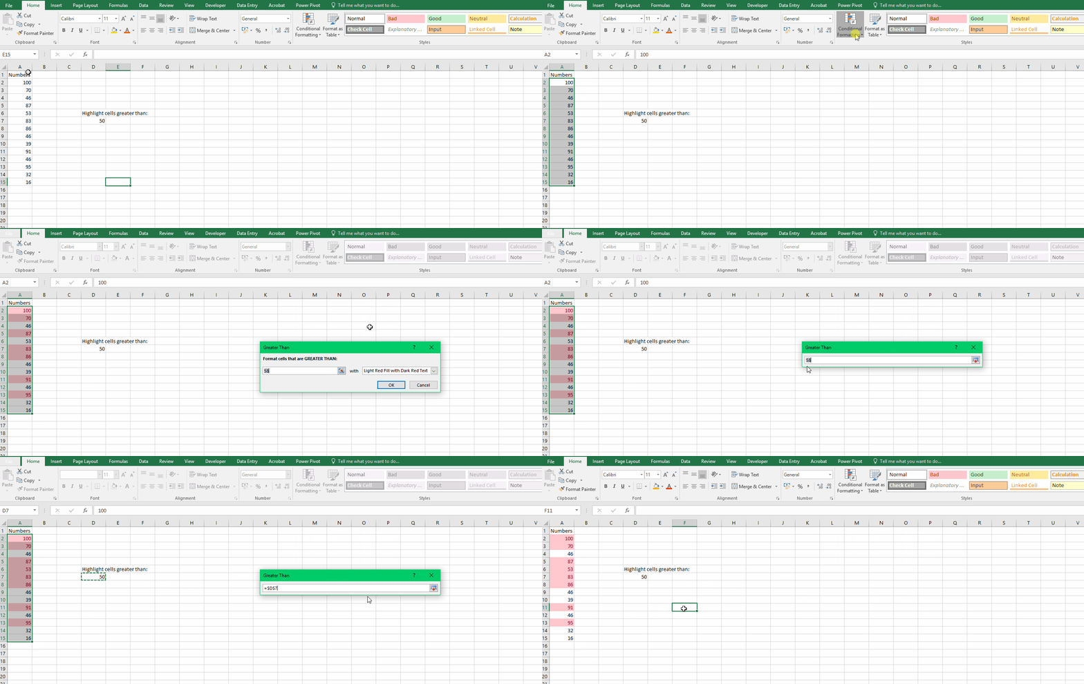
Highlight cells based on criteria such as:- Greater than / Less than
- Between two values
- Equal to a value
- Text that contains specific words
- A date occurring (single date only)
- Duplicate values
Top/Bottom Rules
Highlight:- Top 10 items or Top 10%
- Bottom 10 items or Bottom 10%
- Above or Below Average
Data Bars
Displays a horizontal bar inside the cell proportional to its value. Useful for comparing values at a glance.Color Scales
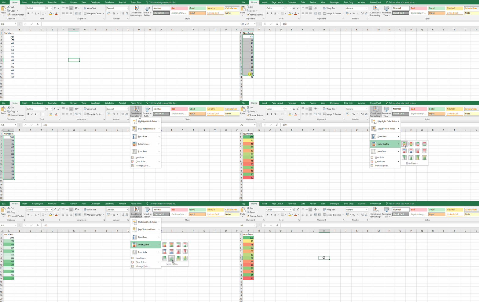
Applies a gradient color based on cell values. Options include 2-color or 3-color scales.Icon Sets
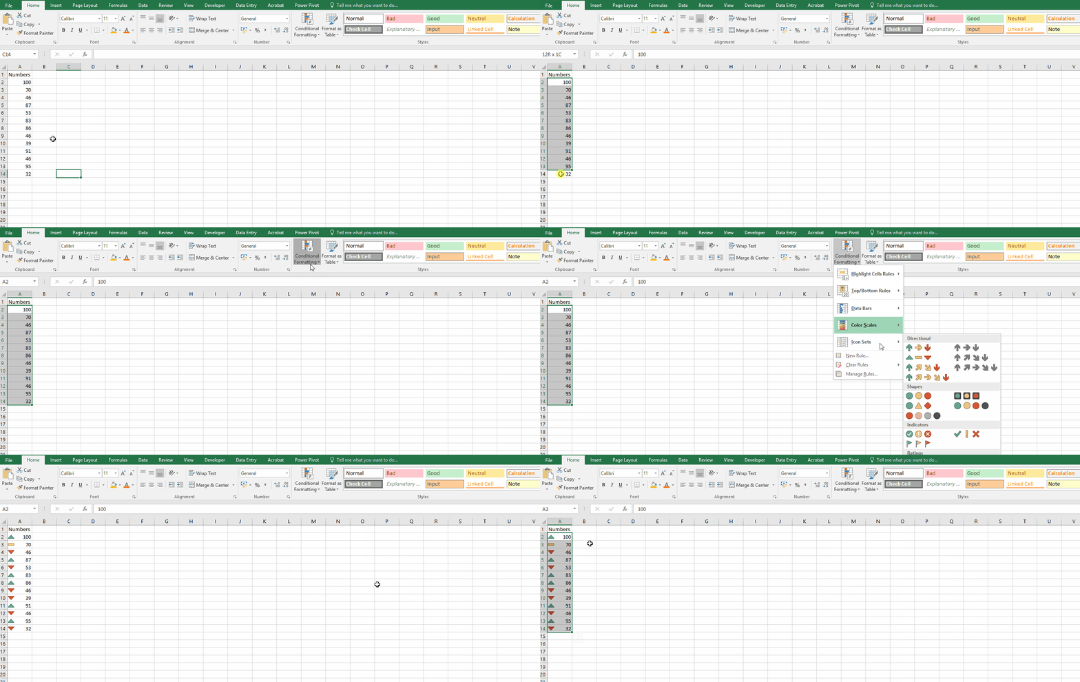
Adds icons (arrows, flags, etc.) to indicate value changes or rankings.
Examples of Each Option #
Highlight Cells Rules: Quickly identify values greater than a threshold.

Top/Bottom Rules: Spot highest or lowest performers.

Data Bars: Visualize relative size of values.

Color Scales: Identify high and low values using color gradients.

Icon Sets: Show trends (up, down, unchanged) with icons.

Creating Custom Rules
If presets don’t meet your needs, you can create custom rules:
- Select the range you want to format.
- Click Conditional Formatting > New Rule.
- Choose a rule type:
- Format all cells based on their value (color scales, data bars, icon sets)
- Format only cells that contain specific criteria (text, numbers, dates)
- Format top/bottom ranked values
- Format above/below average values
- Format unique or duplicate values
- Use a formula to determine which cells to format
Using Formulas #
Formulas allow advanced customization. For example:
=ISBLANK(A1)
Formats cells that are blank.
