VLOOKUP & HLOOKUP
Excel can use lookup functions to retrieve data from a specific column or row within a table.
- VLOOKUP returns a value from a column (vertical).
- HLOOKUP returns a value from a row (horizontal).
Therefore, the V stands for Vertical lookup and the H stands for Horizontal lookup.
Syntax
=VLOOKUP(lookup_value, table_array, col_index_num, [range_lookup])
=HLOOKUP(lookup_value, table_array, row_index_num, [range_lookup])
Arguments
- lookup_value
The value to find in the first column (VLOOKUP) or the first row (HLOOKUP) of the table. This can be a cell reference or typed value.
- table_array
The table where the lookup should happen.- For VLOOKUP, the lookup value must be in the leftmost column of this range.
- For HLOOKUP, the lookup value must be in the top row of this range.
- Col_index_num / row_index_num
- Which column (VLOOKUP) or row (HLOOKUP) to return from within the
table_array. If the index is less than 1 or greater than the number of available columns/rows, you’ll get an error (
#VALUE!or#REF!).
- Which column (VLOOKUP) or row (HLOOKUP) to return from within the
[range_lookup] (optional)
FALSE= Exact match only.TRUEor omitted = Approximate match.- For approximate match, the first column (VLOOKUP) or top row (HLOOKUP) must be sorted ascending; otherwise results may be incorrect
Step by Step: VLOOKUP (Vertical)
- Check your layout
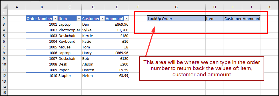
Ensure the value you’re looking up is in the first (leftmost) column of your table. Example: we’ll look up an Order Number to return the linked details using VLOOKUP. - Create your output area
Set aside cells where the returned values should be displayed (e.g., Item, Customer, Status). - Build the function
To return the Item (which sits in the second column of the table), use:=VLOOKUP($F$2, $A$2:$D$100, 2, FALSE)
$F$2contains the Order Number you’re finding.$A$2:$D$100is the table range (Order Number must be column A).2returns from the second column (Item).FALSEensures an exact match
4.Return other fields
In the next cell, change the
col_index_num to return a different column (e.g., 3 for Customer):=VLOOKUP($F$2, $A$2:$D$100, 3, FALSE)
Picture

Exact vs Approximate Match
- Use
FALSEfor IDs, codes, names—anything that must match exactly. - Use
TRUE(or omit the last argument) for banded ranges (e.g., grades, tax bands).- Remember: the lookup column/top row must be sorted ascending for approximate matches; if not, results can be wrong.