Excel has a feature that allows you to format a cell so it can only contain specific answers you’ve defined. These options appear in a drop-down list when the cell is selected. This is useful for reducing spelling errors or typos and helps ensure consistent data entry.
Create Your List of Options
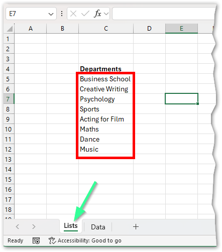
Start by recording all the options you want to appear in the drop-down list. It’s recommended to create this list in a separate worksheet. If the list is deleted later, the drop-down will stop working. If you plan to have multiple lists, you can store them all on the same worksheet, away from your main data.
For example, let’s create a list of University departments:
In a new worksheet, enter your options in a single column (do not include a title in the selection).
Picture
Define a Named Range
Once your list is complete:
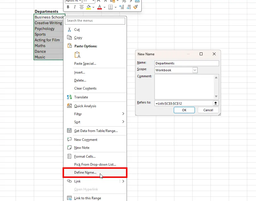
Select the cells containing your options (avoid selecting any header).
Right-click and choose Define Name.
In the dialog box:
Enter a name for the range (e.g., Departments).
Optionally, add comments.
Confirm the cell reference is correct.
Click OK.
Excel will now recognize this range by the name you set. Remember this name for the next step.
Picture
Apply Data Validation
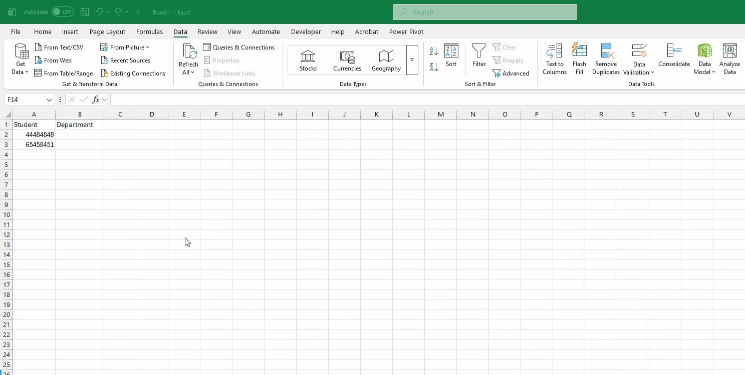
Now, apply the drop-down list to the cells where you want it:
Select the cells (this can be a single cell, a row, a column, or a group of cells).
Go to the Data tab on the ribbon and click Data Validation.
In the dialog box:
Under Allow, select List.
In the Source field, type =Departments (or the name you defined earlier).
If you didn’t define a name, you can reference the range directly, e.g., =A3:A13.
Click OK.
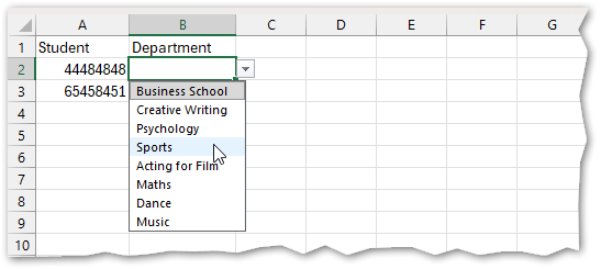
Test Your Drop-Down
Click any cell where you applied data validation. You should now see a drop-down arrow, allowing you to select from your predefined list.